Microsoft Excel is one of the most versatile and popular tools in modern offices. Besides creating simple tables and small databases, there is almost nothing that one can’t achieve by using Excel’s enormous library of functions and extensions. However, Excel’s versatility comes at a price. Mastering Excel completely is near to impossible, due to its vast number of features. Thus, at times, most users are finding themselves employing overly complex features instead of simpler tools that could achieve the same results.
Through this post, we attempt to push your Excel efficiency by demonstrating useful, yet less known, tricks of Excel’s custom formatting.
Custom formatting of numbers:
While working with Excel, you will come across situations where you will have to format numbers and text according to specific necessities. For example, you might want:
- positive numbers to have a ‘+’ sign in front of them,
- negative numbers to be in brackets,
- zero values displayed as empty spaces or a ‘-’ sign,
- numbers to be accompanied by units like meters or kg, while still being able to use them for calculations.
In all such circumstances, the best way forward is using custom formatting. Many users commit the mistake and try to achieve these effects by using conditional formatting because they are well-versed with the conditional formatting tool. However, they usually end up converting their neat Excel sheets into a messy set of diffuse and complicate conditional formatting rules.
How does custom formatting work?
Custom formatting only affects how a value is displayed in a cell – it doesn’t change the actual figure. So you can continue to use it in formulas or search them via vlookup or hlookup.
Let’s take a look at an example:

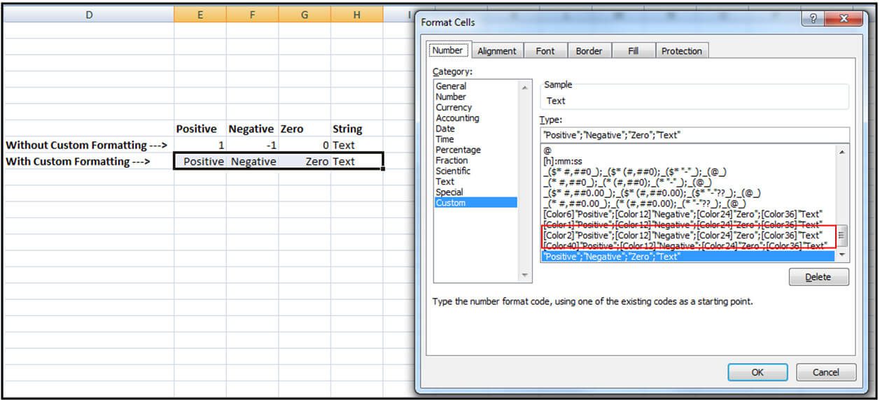
It might be surprising, but Image (1.1) shows two rows with identical content – the difference that you spot, is solely due to the customized format of the second row:
- Positive numbers get displayed as the string ‘Positive’
- Negative numbers get displayed as the string ‘Negative’
- The number 0 gets displayed as the string ‘Zero’
- Plain text remains plain text
How to do it:
Select the cell or range that you want to format. Right click to open the menu and select ‘format’. After these steps, choose the category ‘custom’ in the ‘Number’ tab. Here you can change the type by selecting one of the listed, predefined options or by defining your own.
You can specify up to four format treatments: one for all positive numbers, one for all negative numbers, one for the value 0 and one for plain text. Excel interprets the cases always in this specifc order and only if separated by ‘;’.
There are several possibilities to format numbers. A good overview provided by Microsoft can be found here https://support.office.com/en-us/article/Number-format-codes-5026bbd6-04bc-48cd-bf33-80f18b4eae68 but I will also provide a short summary:
| To display | As | Use this code |
|---|---|---|
| 1234.59 | 1234.6 | ####.# |
| 8.9 | 8.9 | #.000 |
| 0.631 | 0.6 | 0.# |
| 12 | 12 | #.0# |
| 1234.568 | 1234.57 | |
| Number: | Decimal points aligned: | ???.??? |
| 44.398 | 44.398 | |
| 102.65 | 102.65 | |
| 2.8 | 2.8 | |
| Number: | Numerators of fractions aligned: | # ???/??? |
| 5.25 | 5 1/4 | |
| 5.3 | 5 3/10 |
To display a comma as a separator in thousand or to scale a number by a multiple of 1000, include a comma (,) in the code for the number format.
| To display | As | Use this code |
|---|---|---|
| 12000 | 12,000 | #,### |
| 12000 | 12 | #, |
| 12200000 | 12.2 | 0.0,, |
To display leading and trailing zeros prior to or after a whole number, use the codes in the following table.
| To display | As | Use this code |
|---|---|---|
| 12 | 00012 | 00000 |
| 12 | 00012 | "000"# |
| 123 | 0123 | "0"# |
- 1234.59 as 1234.6
- -1234.59 as ‘neg’
- 0 as ‘-‘
- leave plain text unchanged.
Color formatting in Excel:
Another Excel functionality of great importance is the application of different colors to the content of cells. For instance, make the font color of negative numbers ‘red’ or the color of positive numbers ‘green’.
You can assign different colors to each of the four cases mentioned above: positive numbers, negative numbers, value 0, and plain text. Again, you have to specify the case in this fixed order and separate them by ‘;’.
For example, the formatting code ‘[Red]General;[Green]General ;[Yellow] General;[Blue] General’ would display all positive numbers green, negative numbers red, 0 values yellow, and text blue.
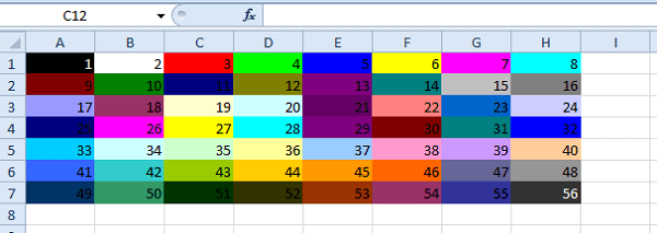
All Excel versions support common colors like Black, Green, White, Blue, Magenta, Yellow, Cyan and Red. It is also possible to use the color number instead of the color name provided by Excel straight from 0 to 56 (see the image given below).

By using the color codes our simple example above could also be written as ‘[Color 3]General;[Color 4]General ;[Color 6]General;[Color 5]General‘
Scaling Values:
One comes across the issue to convert absolute numbers in different scaling categories, especially when reporting financial results. Rather than resorting to Excel formulae, we can sort out this problem by applying custom formatting again. Let’s take a look at an example.
| Scaling in ? | Absolute value | Excel formulae | Custom Formatting | Custom Trick |
|---|---|---|---|---|
| In Thousands | 12000000000 | 12000000 | 12000000 | ###0.00, |
| In Hundreds | 12000000000 | 120000000 | 120000000 | ####"."00 |
| In Millions | 12000000000 | 12000 | 120000 | ####.00,, |
| Adding Zero | 12000000000 | 1.2E+12 | 1.2E+12 | ####"00".00 |
| Showing in the form of Ratio | 1.8 | 1.8x | 1.80x | #0.00"x" |
| Showing in the form of Fraction | 2.1 | 2 5/50 | # ??/50 |
All cells in the upper part of the table carry the number 12000000000.00. By adding a single comma “,” we display this rather large number in thousands or by adding ‘,,’ in millions. Displaying fractions (last two rows) isn’t possible without custom formatting at all.


